Lab 11: mmWave FMCW Sensing IoT

Date: July 21
Lab window: 1:00-5:00 PM
TA: Shanmu Wang
Format: Groups of 4
Hardware: One IWRL6432FSPEVM Evaluation Module per group

Goals

By the end of this lab, each group should be able to:

• explain how FMCW radar converts echo delay into range;
• read range-profile and point-cloud data from the TI xWRL6432/IWRL6432 demo firmware;
• implement simple background subtraction for range profiles;
• detect a hand or moving reflector in front of the radar;
• visualize point-cloud returns and compare them with range-profile measurements;
• collect a small mmWave sensing dataset;
• train and evaluate at least one simple classifier for a radar sensing task.

Hardware

Form a group of 4 in the class sheet:

Open mmWave group sheet

The IWRL6432FSPEVM is a compact 60 GHz mmWave radar evaluation kit based on TI’s IWRL6432 radar device. For this lab, we use the preflashed mmwDemo firmware and communicate with the board over a USB-to-UART adapter.

Item	Value
Radar band	57-64 GHz
Antennas	2 transmit antennas, 3 receive antennas
Field of view	120 degrees azimuth, 80 degrees elevation
Host/data interface used in lab	UART
Demo firmware used in lab	Preflashed xWRL6432 mmwDemo
Core processing	Arm M4F plus TI Radar Hardware Accelerator for FFT, log magnitude, and CFAR

Official references:

• IWRL6432FSPEVM Evaluation Module User’s Guide
• IWRL6432 datasheet
• IWRL6432FSPEVM product page
• MMWAVE-L-SDK

Repository

Use the course mmWave lab repository:

Open mmWave lab repository

Each group member should fork the repository and clone their own fork.

git clone https://github.com/YOUR_GITHUB_USERNAME/mmwave_lab.git
cd mmwave_lab
git checkout student-todo
conda activate cosmos-ds

Search for TODOs:

rg TODO

If rg is not installed, use VS Code global search with Ctrl+Shift+F on Windows/Linux or Cmd+Shift+F on macOS and search for TODO.

The main student TODOs are in:

• hand_lab.py
• hand_motion_lab.py
• plot_posture_classifier_accuracy.py, if your group chooses the posture track

Big Picture

The data path in this lab is:

radar chirps
  -> received echoes
  -> demo firmware range / point-cloud processing
  -> UART TLV packets
  -> Python parser and visualization
  -> background subtraction, features, and ML

The lab starts with hand-range and moving-target experiments so you understand the signal. Then each group uses the same radar stream for one application track, such as box presence detection or posture recognition.

Step Index

1. Connect the radar board with the USB-to-UART convertor.
2. Find the USB serial port.
3. Run the hand range experiment.
4. Complete range-profile background subtraction TODOs.
5. Run moving-target detection.
6. Visualize point clouds and near-field returns.
7. Choose one application track.
8. Collect a dataset.
9. Train and evaluate a classifier.
10. Prepare checkoff answers.

Section 1: Hardware Setup

Step 1: Wire the EVM in Functional Mode

Use swru628.pdf Section 2.3 as the board reference. Handle the EVM carefully and keep people at least 5 cm from the radar during operation.

Required hardware:

• IWRL6432FSP/xWRL6432 EVM;
• 1.27 mm to 2.54 mm breakout board from the kit;
• USB-to-UART adapter with 3.3 V logic;
• female-to-female Dupont jumper wires;
• micro-USB cable from the USB-to-UART adapter to the computer.

Wire the radar breakout to the USB-to-UART adapter:

Radar breakout pin	USB-to-UART pin	Notes
3V3	SYS3V3	Powers the radar board from USB 3.3 V.
GND	GND	Common ground.
UART RX	TXD	TX/RX are crossed.
UART TX	RXD	TX/RX are crossed.
SOP1	GND	Required for functional mode.
SOP0	3V3	Functional mode for the preflashed demo.

Do not connect SOP0 to GND for this lab. That is flashing mode. Power-cycle the board after changing SOP wiring.

The image step-by-step tutorial is as follows:

1. Connects the male-to-female Dupont Wires to the convertor:

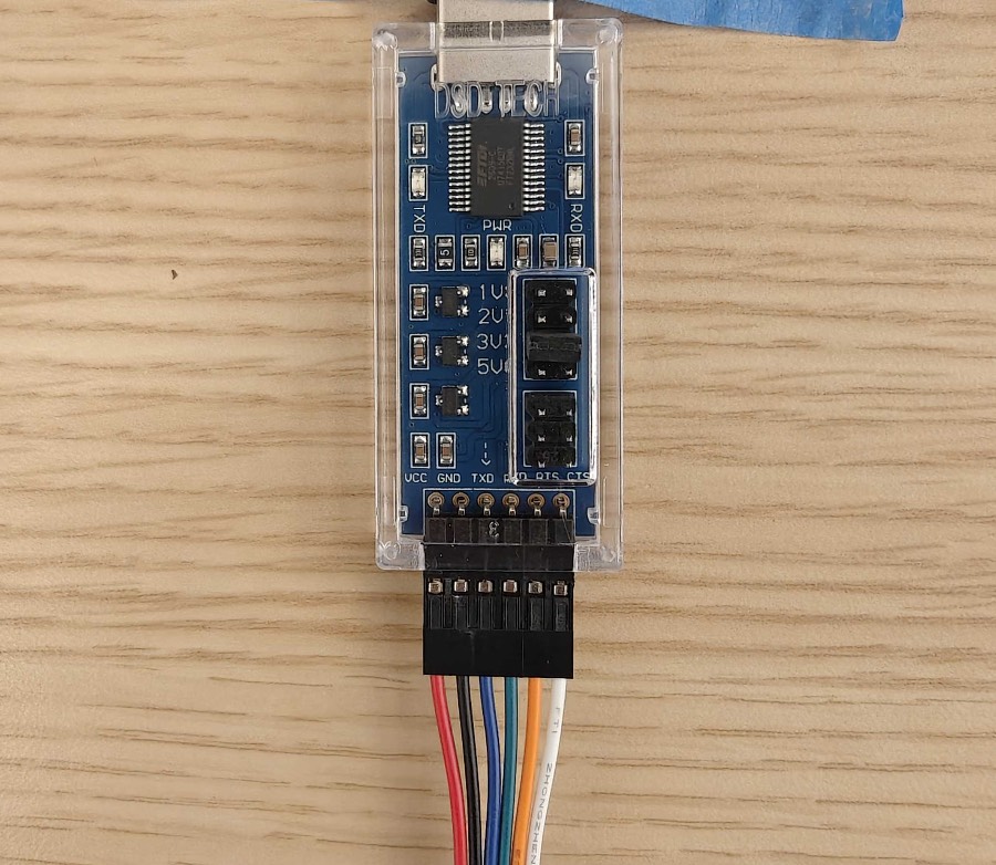
2. Split the left 4 wires (Red, black, blue, and green) and connect them to the radar board:

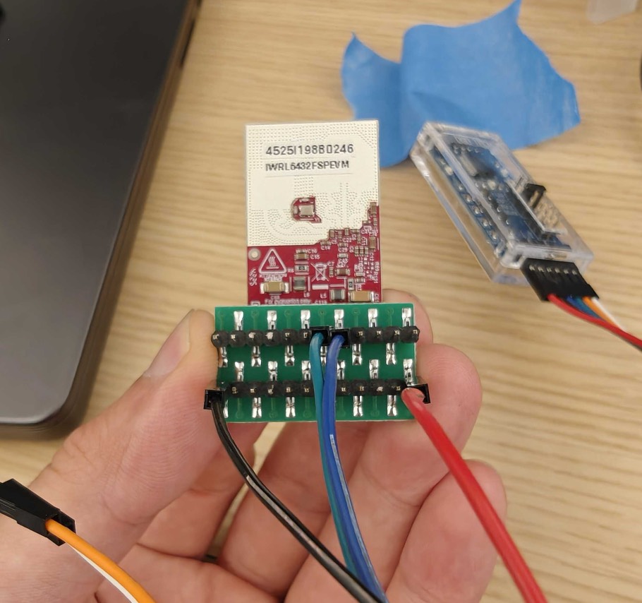
3. Then connects the board with 2 female-to-female Dupont Wires:

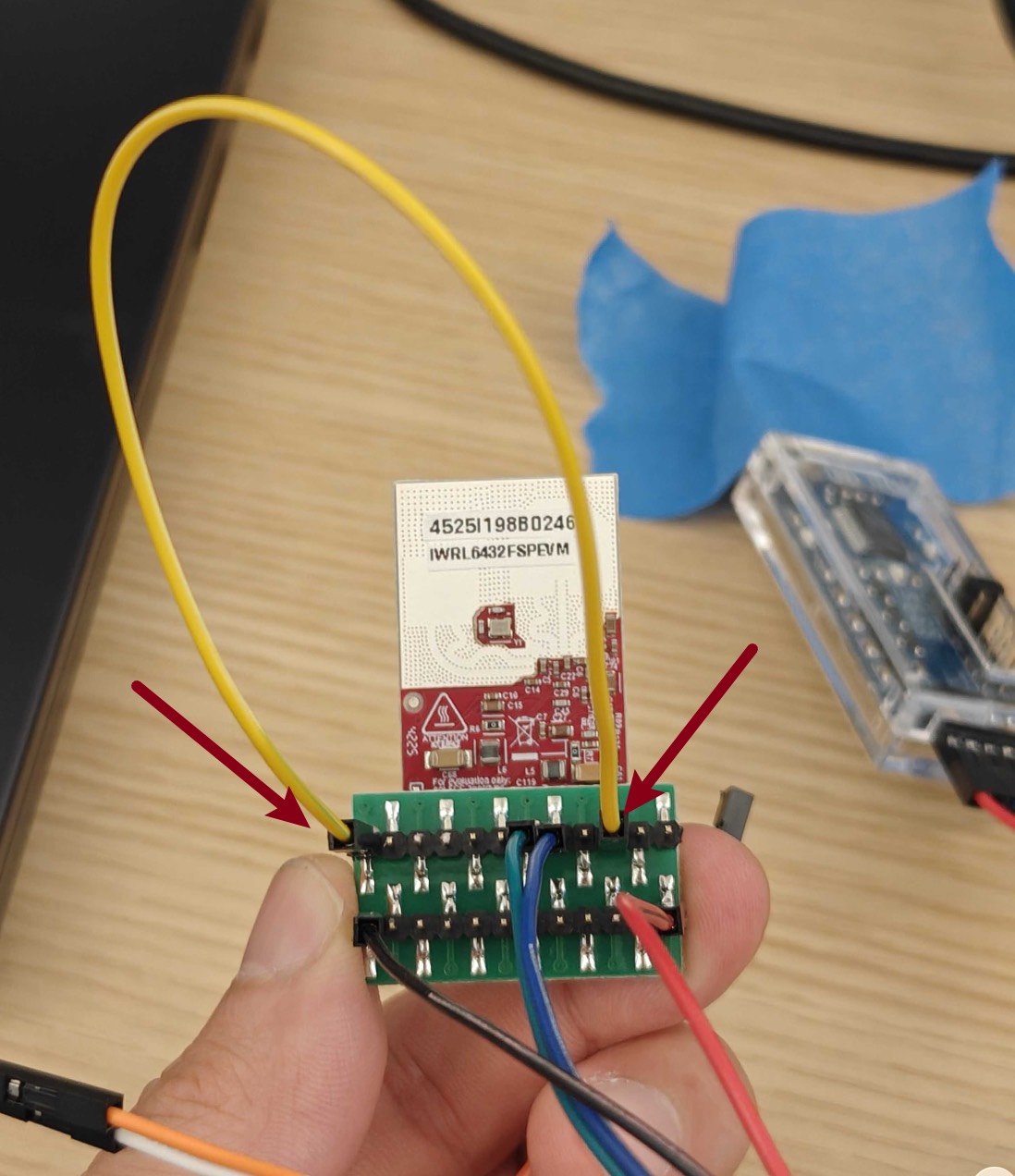
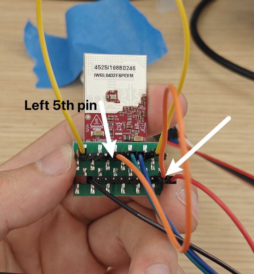
Step 2: Find the Serial Port

Use the serial port from the USB-to-UART adapter in all commands below.

macOS:

ls /dev/cu.usbserial* /dev/cu.usbmodem* 2>/dev/null
python -m serial.tools.list_ports -v

The port usually looks like:

/dev/cu.usbserial-BH00LV2S
/dev/cu.usbserial-5B1F0090131

Use the /dev/cu... device, not /dev/tty....

Windows:

Device Manager -> Ports (COM & LPT)

In the commands below, replace <PORT> with your actual port, for example /dev/cu.usbserial-BH00LV2S on macOS or COM5 on Windows.

Section 2: FMCW Range Profile

FMCW radar transmits chirps whose frequency ramps over time. A delayed echo mixes with the current transmit signal and produces a beat frequency. For chirp slope S, beat frequency f_b, and speed of light c, a simplified range estimate is:

R = c * f_b / (2 * S)

The range FFT separates beat frequencies into range bins. In this lab, hand_lab.py reads range-profile TLVs from the demo firmware and asks you to finish the processing.

Step 3: Run the Hand Range Experiment

From the mmwave_lab repository:

python hand_lab.py --port <PORT>

Procedure:

1. Keep the area in front of the radar empty while the first background frames are captured.
2. Put one hand in front of the radar.
3. Move the hand slowly between about 15 cm and 1 m.
4. Watch the printed distance and the background-subtracted range plot.

Useful options:

python hand_lab.py --port <PORT> --background-frames 40
python hand_lab.py --port <PORT> --min-range 0.2 --max-range 2.0
python hand_lab.py --port <PORT> --no-db

Step 4: Complete the Hand-Range TODOs

Open hand_lab.py and finish the TODOs:

1. Collect N empty-scene range profiles.
2. Compute the background as the median profile.
3. Subtract the background with max(profile - background, 0).
4. Find the strongest peak inside a valid range window.
5. Convert the peak bin index to meters.
6. Smooth the distance over the last few estimates.

Implement both mean smoothing and median smoothing, then decide which one is more robust when one frame has a bad peak.

Checkoff questions:

1. Why do we collect an empty-scene background before detecting the hand?
2. Why is the median background often better than using one raw frame?
3. Which smoothing method was more stable for your group, mean or median?

Section 3: Moving-Target Background Subtraction

A static background removes clutter that was already present during calibration. Moving-target detection uses a background that slowly updates over time.

Step 5: Run the Moving-Target Lab

Run:

python hand_motion_lab.py --port <PORT>

Procedure:

1. Keep the scene still while the first frames initialize the background.
2. Move one hand or a reflector in front of the radar.
3. Watch the moving-target range estimate and waterfall plot.
4. Try several --alpha values.

Useful options:

python hand_motion_lab.py --port <PORT> --alpha 0.01
python hand_motion_lab.py --port <PORT> --residual positive
python hand_motion_lab.py --port <PORT> --history-frames 120
python hand_motion_lab.py --port <PORT> --no-db

Student TODO in hand_motion_lab.py:

background = (1 - alpha) * background + alpha * profile

Checkoff question: what is the tradeoff between a small alpha and a large alpha?

Section 4: Point Cloud and Near-Field Visualization

The firmware can also report detected point clouds. A point cloud is already a compressed representation: the radar has performed range/Doppler/antenna processing and detection, then reports only selected points.

Step 6: Run the Point-Cloud Viewer

Run:

python point_cloud_viewer.py --port <PORT> --cfg xwrL64xx-evm/point_cloud.cfg

Move a reflector left/right and nearer/farther from the radar. The viewer is a top-down x/y display:

• x: left/right position;
• y: forward range.

The preflashed demo often reports raw z near zero, so this lab treats point clouds as 2D.

Color options:

python point_cloud_viewer.py --port <PORT> --color-by range
python point_cloud_viewer.py --port <PORT> --color-by velocity

Step 7: Compare Near-Field Range and Point Clouds

For near-field hand and reflector motion, run:

python near_field_gesture_viewer.py --port <PORT>

This viewer shows:

• the first 50 cm of the background-subtracted range profile;
• a rolling range waterfall;
• the front-region point cloud, restricted to about +/-15 cm in x and less than 50 cm in y.

To inspect the raw range profile without subtraction:

python get_range_profile.py --port <PORT> --cfg xwrL64xx-evm/hand_distance.cfg

Compare the raw range profile with the background-subtracted displays.

Checkoff questions:

1. What static objects appear in the raw range profile?
2. What changes after background subtraction?
3. What information is lost when raw radar returns are reduced to a point cloud?

Section 5: Application Track

Choose one or both application tracks. Both the box-presence track and the posture track are easy and similar to previous labs. So I personally recommend do both. If your group only wants to do one of them, the posture one might be more interesting.

Track A: See Through the Box, Empty vs Object

Goal: classify whether a closed box is empty or contains a strong reflector, such as a phone.

Use the same box for both classes. Keep the radar and box position as fixed as possible. For each object recording, put the reflector inside the closed box and slowly move or rotate the box during capture. For each empty recording, close the same box with nothing inside and move it in a similar way.

Step 8A: Collect Box-Presence Data

python collect_box_presence_dataset.py --port <PORT> --trials 3

The script collects two labels:

• empty: closed empty box;
• object: closed box with a reflector inside.

The first calibration captures the empty scene with no box in front of the radar. The same background is saved in the dataset folder as background.npz.

Short smoke test:

python collect_box_presence_dataset.py --port <PORT> --trials 1 --duration 10

Step 9A: Train the Box-Presence Classifier

python train_box_presence.py datasets/box_presence_dataset_YYYYMMDD_HHMMSS

The default classifier is a random forest. Training cuts each 60-second recording into 2-second segments with 50% overlap. The default feature is a background-subtracted dB range image resampled to 24 x 32.

Useful options:

python train_box_presence.py DATASET --classifier random_forest
python train_box_presence.py DATASET --classifier svm_rbf
python train_box_presence.py DATASET --classifier knn
python train_box_presence.py DATASET --max-range 0.80 --resample-frames 24 --resample-bins 32

Use the default recording-level split for real evaluation. Use --allow-segment-split only for quick code smoke tests, because overlapping windows from the same recording can make accuracy look unrealistically high.

Step 10A: Evaluate Box Presence in Real Time

python eval_box_presence_realtime.py \
  --model datasets/box_presence_dataset_YYYYMMDD_HHMMSS/models/random_forest_box_presence_YYYYMMDD_HHMMSS.joblib \
  --port <PORT>

If the radar setup has not moved since data collection, use the same saved background:

python eval_box_presence_realtime.py \
  --model MODEL.joblib \
  --port <PORT> \
  --background-npz datasets/box_presence_dataset_YYYYMMDD_HHMMSS/background.npz

More detail: BOX_PRESENCE_PIPELINE.md.

Track B: Posture Recognition

Goal: classify human posture using the top-down point cloud.

Default posture labels:

• empty: no person in front of the radar;
• sitting: person sitting;
• standing: person standing naturally;
• standing_arms_forward: person standing with both arms extended straight forward;
• squat: person squatting or crouching.

Step 8B: Collect Posture Data

Each student should use a unique collector ID:

python collect_posture_dataset.py \
  --port <PORT> \
  --collector student01 \
  --trials 3

Short smoke test:

python collect_posture_dataset.py \
  --port <PORT> \
  --collector student01 \
  --trials 1 \
  --duration 10

Each trial records a continuous point-cloud stream. Important arrays include:

• points_xyz: NaN-padded firmware point cloud;
• points_velocity: NaN-padded point velocity;
• point_count: valid point count per frame;
• time_s: frame timestamps.

Step 9B: Combine and Train

After each student collects data, combine the dataset folders:

python combine_posture_datasets.py \
  datasets/posture_dataset_STUDENT_A \
  datasets/posture_dataset_STUDENT_B \
  datasets/posture_dataset_STUDENT_C \
  --output datasets/combined_posture_all_students

Train:

python train_posture.py datasets/combined_posture_all_students

Training cuts each recording into 2-second segments with 50% overlap. Features are computed from the top-down point cloud: point count over time, x/y centroid and spatial extent, body width/depth, and x/y occupancy over time.

Useful options:

python train_posture.py DATASET --classifier random_forest
python train_posture.py DATASET --classifier knn
python train_posture.py DATASET --classifier svm_rbf
python train_posture.py DATASET --classifier decision_tree
python train_posture.py DATASET --group-by collector

Student TODO after the first model works:

1. Train at least three classifiers.
2. Repeat each classifier with several random seeds.
3. Complete plot_posture_classifier_accuracy.py.
4. Plot average validation accuracy for each classifier.
5. Use the plot to justify which model should be used for real-time evaluation.

Run the completed plotting helper like this:

python plot_posture_classifier_accuracy.py DATASET/models/*.joblib

Step 10B: Evaluate Posture in Real Time

python eval_posture_realtime.py \
  --model datasets/combined_posture_all_students/models/random_forest_posture_YYYYMMDD_HHMMSS.joblib \
  --port <PORT>

More detail: POSTURE_PIPELINE.md.

Finish the squat_couter_gui.py and see the squat couter with your trained model:

    def update(self, stable_label: str | None, time_s: float) -> str:
        """Advance standing -> squat -> standing state machine."""
        if stable_label is None:
            return ""

        label = str(stable_label)
        if label not in {self.standing_label, self.squat_label}:
            return ""

        if self.state == "wait_for_standing":
            if label == self.standing_label:
                self.state = "standing_ready"
                return "ready"
            return ""

        if self.state == "standing_ready":
            if label == self.squat_label:
                self.state = "in_squat"
                return "down"
            return ""

        if self.state == "in_squat":
            if label == self.standing_label:
                if time_s - self.last_count_time_s >= self.min_count_interval_s:
                    self.count += 1
                    self.last_count_time_s = time_s
                    self.state = "standing_ready"
                    return "count"
                self.state = "standing_ready"
                return "too_soon"
            return ""

        self.state = "wait_for_standing"
        return ""

Optional Track C: Static Box Contents

If your group finishes early, try the multi-class box-content task.

Collect:

python collect_box_dataset.py --port <PORT> --contents empty,board,marker_pen,phone --trials 8

Train:

python train_box.py datasets/box_contents_dataset_YYYYMMDD_HHMMSS

Evaluate:

python eval_box_realtime.py \
  --model datasets/box_contents_dataset_YYYYMMDD_HHMMSS/models/random_forest_box_contents_YYYYMMDD_HHMMSS.joblib \
  --port <PORT>

More detail: BOX_CONTENTS_PIPELINE.md.

Checkoff and Submission

Show the TA:

1. Correct functional-mode wiring: SOP0 -> 3V3, SOP1 -> GND.
2. The serial port used by your group.
3. hand_lab.py reporting a reasonable hand distance after your TODOs are implemented.
4. A comparison of mean vs median smoothing for hand distance.
5. hand_motion_lab.py running with your exponential background update.
6. A point-cloud or near-field viewer screenshot.
7. One application-track dataset folder.
8. One trained model and its evaluation output.
9. One live prediction demo, if your model is ready.

Submit or paste into your group notes:

1. Group members and hardware setup notes.
2. Serial port name.
3. Answers to the hand-range and moving-background checkoff questions.
4. A screenshot of the range profile or waterfall.
5. A screenshot of the point-cloud or near-field viewer.
6. Which application track you chose.
7. Dataset labels and number of trials.
8. Classifier type and validation accuracy.
9. One paragraph explaining what made the task hard.

Troubleshooting

Problem	Likely cause	Fix
No serial port appears	USB cable, adapter, or driver issue	Reconnect the adapter, try another cable, and install the FTDI USB-to-UART driver if needed.
Script cannot configure the radar after a previous run	The demo is still running or in an old CLI state	Press reset or power-cycle the EVM, then rerun the script.
CLI reports a DPU or configuration error	Wrong SOP wiring or stale low-power state	Confirm functional mode: SOP0 -> 3V3, SOP1 -> GND; power-cycle the board.
No hand peak appears	Background captured with hand present, wrong range window, or weak reflection	Recalibrate with empty scene, move the hand into 15 cm to 1 m range, and adjust --min-range / --max-range.
Moving target disappears too quickly	alpha is too large	Try a smaller --alpha.
Live classifier is stuck on one class	Too little data or biased collection	Collect more trials, interleave labels, and keep motion/setup consistent across classes.
Accuracy is suspiciously high	Segment leakage from the same recording	Prefer recording-level or collector-level splits instead of segment-level smoke tests.

Use Ctrl+C to stop live scripts. The scripts try to send sensorStop 0 before exiting.

Core Takeaway

mmWave radar can be used as a sensing signal, not only as a distance sensor. In this lab, range profiles and point clouds are first inspected directly, then transformed with background subtraction and machine learning into application-level predictions.